Beauty Behind Chaos: Newton's Fractal
In mathematics, regardless if you’re studying it in school or at your job as a physician or computer scientist, we deal with “algorithms” that seemingly generate results based on a set of inputs. Generally, we focus on the micro aspect on such calculations and prize the numeric result we get. It is a much more “pragmatic” approach, where one cares about solving an equation rather than understanding its structure as a whole.


Newton’s Method’s illustration stems from looking at the macro aspect of an algorithm, which we refer to as “equations” or “functions” in mathematics. Rather than being concerned about singular results, it attempts to explain the behavior of an approximation algorithm which in real life might not initially have much use. As a result, topics like this are generally disregarded in applied mathematics, where understanding the why and how is usually less important than the result.
To explain this seemingly chaotic but also beautiful image, I first have to explain this “pragmatic” and seemingly unrelated algorithm that I was referring to. It is Newton’s Approximation Algorithm, which physician Isaac Newton developed to precisely approximate the roots of high-degree polynomials. To make sense of this perplexing fractal, we first need to understand the rather simple workings of Newton’s Methods.
A Brief Intro to Newton’s Methods
We’ve all been introduced to polynomials, where they are in the rather simple form of:
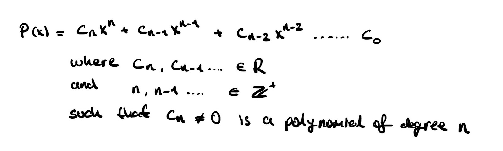
The simple algebraic notation and properties of polynomials make it a pivotal tool in engineering and physics in general. They are used everywhere ranging from computer graphics to determining the state of moving objects. Specifically, one of the most important properties of polynomials are their zeros: where P(x) = 0. We have the famous quadratic equation to calculate these values for a polynomial of degree 2.
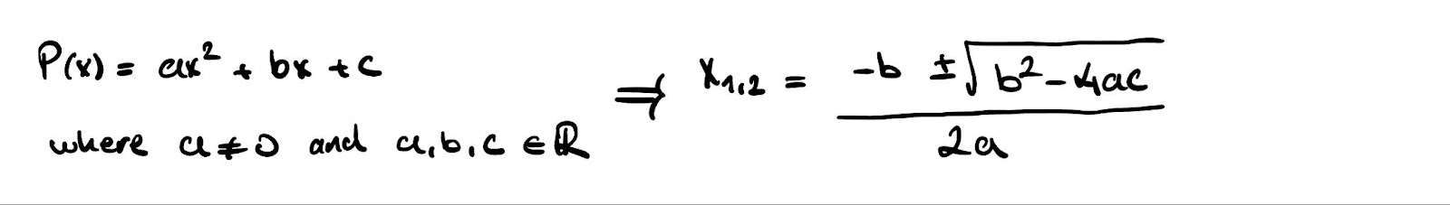
We can trivially calculate these values with this simple formula. But, what about a polynomial of degree 3? How can we formulate a way to calculate the zeros of an arbitrary 3rd degree polynomial? Well, there is a way, but it is nowhere near trivial as the quadratic formula.

As can be seen, it keeps getting harder and harder, and the formula for degree 4 takes up a whole page. And on top of that, there is no formula for a 5 degree polynomial.
Now why might finding the roots of a 5-degree (or any other high-degree) polynomial be necessary? To perhaps make you care, let’s refer to the originator of the method, the father of classical mechanics: Newton. During his studies of natural sciences, he was concerned with the motion of moving bodies. To analyze them, he mathematically formulated their attributes to describe their movements in space.
Let’s say, speaking of polynomials of degree 5, that he reached a formula in the form of a 5th-degree polynomial characterizing the velocity of an object over time. To find the point at which the object is at rest, he has to find the zeros of said polynomial. However, there is no trivial way of doing so. Therefore, he developed the following approximation formula. Let’s work off a concrete example:
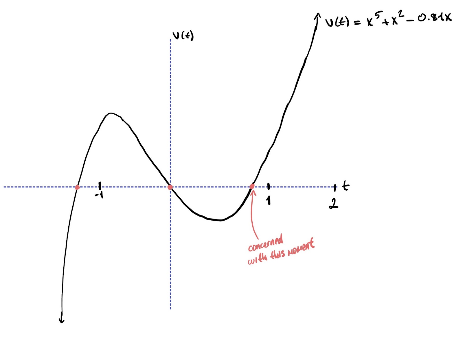
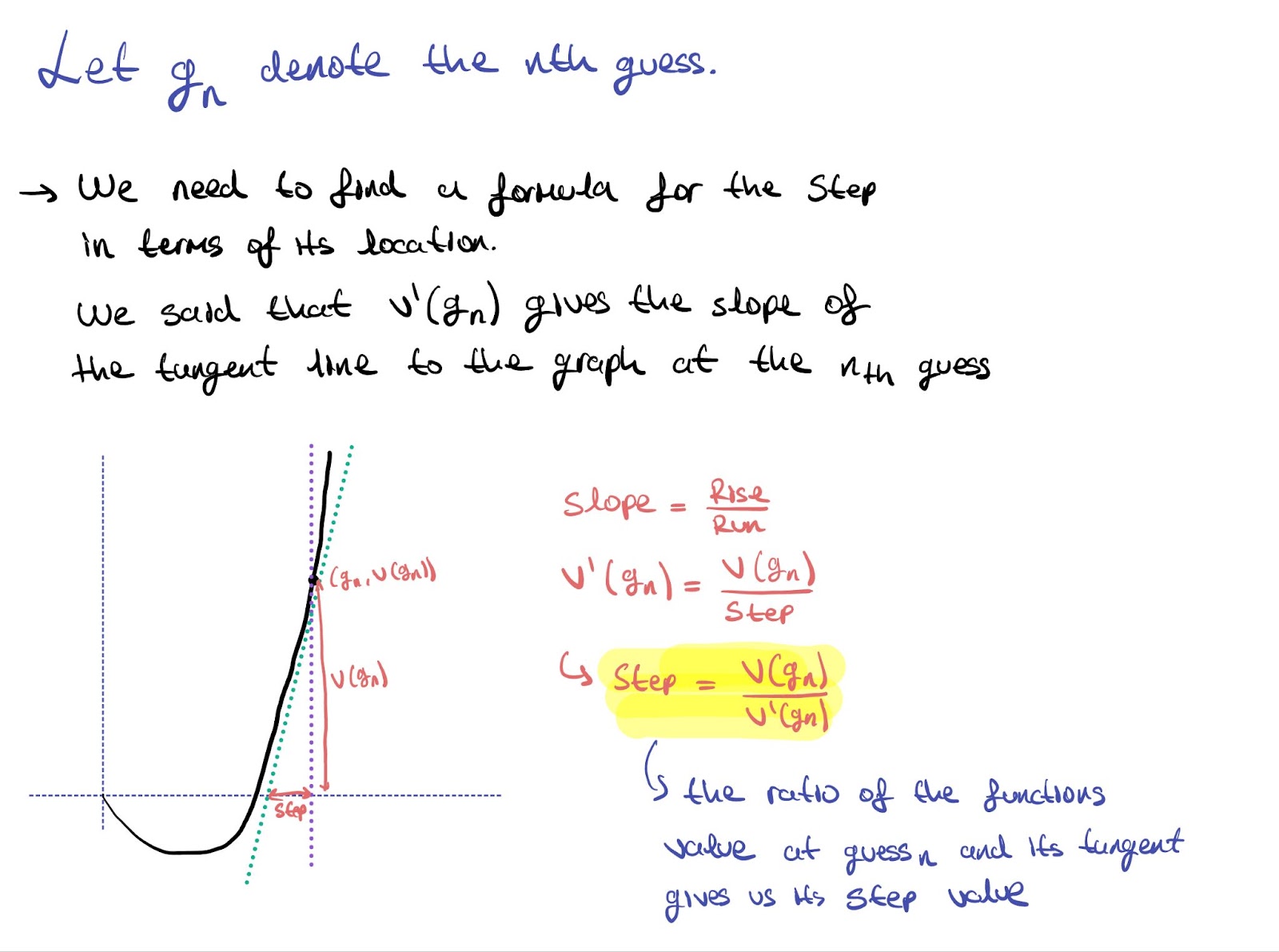
Suppose that we want to find the time value of the marked point. We’ll eyeball a time value close enough to the point that we’re trying to reach, and step towards it to the zero that we are concerned about. Newton’s algorithm relies (this will be important later on with its connection with the fractal) on the fact that we’ve eyeballed a good enough value that is close to the zero we’re concerned about.
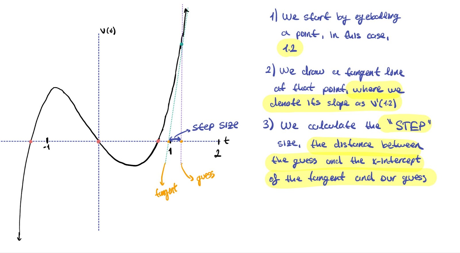
Imagine yourself taking this step on the number line. Now, you’ve landed on your new, second, guess which is closer to your zero of the polynomial. Initially, you were (Guess) - (Zero) away from your desired value. Now, you’ve taken a step towards the zero from your initial guess, and reached a new guess of (Guess - Step), which is now (Guess - Step) - (Zero) away from your zero value! You are getting closer. We can formulate, depending on the guess that we’re taking, the step size that we should take to get closer to our desired value.
Now, finalizing our approximation method, we incorporate the step size with the guess values.
Now that we’ve established how Newton precisely approximated the roots of high-degree polynomials, we can now look at the seemingly unrelated relationship between this and the fractal. Before introducing this method, I’ve placed great emphasis on two things:
- this method works properly for values eyeballed close to the zeros
- this method is not concerned with guesses far away from the zero: it is pragmatic. Newton himself was actually not aware of the existence of the fractal. He merely used it as a “tool” to calculate the zeros; he did not analyze the behavior of his method. So, for approximating a given zero of a polynomial, what happens if our guest value is far away from the value that we’re trying to approach? What happens for ALL guesses? To discuss this, I need to introduce the idea of a “fractal briefly”.
The Fractal
Fractals are “images” drawn on the complex plane, where it allows for analysis of every single number (both real and complex) how it prompts the function being analyzed to behave. The colors are used as “gradients”, indicating to what degree the value causes the function to diverge to a random value, or how it converges. Every point on the complex plane is given a “gradient of color” based on these characteristics, and the numbers attributed with these colors form these beautiful shapes. To think of this in a more concrete way, let’s look at Newton’s Fractal:
Every single dot represents the possibility of all guesses, and as they “march” by taking steps using Newton’s algorithm, some are able to converge towards the zeros. However, some take on different routes and diverge from the zeros. By labeling each dot with the degree on how much it converges or diverges, we are able to plot for every single number (again, both complex and real) how this algorithm behaves. It allows us to see in which patterns it works. Rather than going, “oh, why did it arbitrarily not work this time?”, it allows us to geometrically interpret the pattern behind its convergence or divergence.
These fractals also contain “infinite detail”, where you can zoom in at magnitudes of 10-20and beyond. Connecting this with the “coloring” information above, moving the value of an initial guess by only a value of, let’s say 10-20 can drastically change the outcome. Since the shapes are still preserved in such small magnitudes, a change so small in those magnitudes would still make it very possible for the value to land on a shaded area which symbolizes divergence. It is like a landmine: where without exploring it through fractals, you have no clue of the pattern for the functions behaviour.
At first, a seemingly simple algorithm for approximating roots actually has an intricate behaviour containing infinite detail, only revealed when plotted as a fractal. This emphasizes the difference between applied and pure mathematics. Applied mathematics, like Physics and Engineering is generally concerned with obtaining a result and moving on. Through the mentality of “don’t touch it if it works”, they aim for the fastest and easiest solutions that they can achieve. However during this process, the beauty of mathematics is lost. Mathematics is concerned with generalizing structure, and through this fractal, the approximation methods behaviour was modelled, which turned out to be beautiful.
There are many more fractals like this with completely different underlying functions, but their main principles are the same: modelling the degree of “chaos” (convergence or divergence) of every single number for a function.
Explore numerous fractals here: https://mandelbrotandco.com/newton/index.html
to, Contributors. “Boundary Set in the Complex Plane.” Wikipedia.org, Wikimedia Foundation, Inc., Feb. 2006, en.wikipedia.org/wiki/Newton_fractal. Accessed 18 Feb. 2025.
“3Blue1Brown - Newton’s Fractal (Which Newton Knew Nothing About).” 3blue1brown.com, 2021, www.3blue1brown.com/lessons/newtons-fractal. Accessed 18 Feb. 2025.